TPC-H Walkthrough

A hands-on walkthrough that builds a working Honeydew on top of the TPC-H benchmark: a semantic model, a curated domain, a context layer for the AI, an agent, a BI tool live on the domain, and AI Deep Analysis answering questions on the same model. You can write the YAML by hand, build it in Honeydew Studio, or let a coding agent do the typing through the Honeydew MCP server. The output is the same either way.

Where you’ll end up

By the end:

A semantic model with customer, orders, lineitem, part, partsupp, supplier, nation, and region, plus reusable metrics like revenue
A domain that exposes a curated slice of the model
A context layer with one skill and one event
An agent pairing the domain with that context
A BI tool (Power BI, Tableau, Excel, etc.) live on the domain
Deep Analysis answering investigative questions on the same model

What you’ll need

A Honeydew workspace. Sign up or follow initial setup.
A connected warehouse with the TPC-H schema available.
TPC-H sample data is built into Snowflake (SNOWFLAKE_SAMPLE_DATA.TPCH_SF1) and Databricks (samples.tpch).
Optional, recommended: a coding agent connected to the Honeydew MCP server with the Honeydew plugin for coding agents. Claude Code, Cursor, VS Code, Gemini, Codex, and other agents all work.

The reference model lives at github.com/honeydew-ai/tpch-demo. Fork it to follow along, or build the same thing in your own workspace.

The data

TPC-H is an order-management benchmark that database engines have been competing on for decades. Customers place orders made of line items, parts come from suppliers, customers and suppliers belong to nations, and nations roll up into regions. Orders span six years, starting 1992.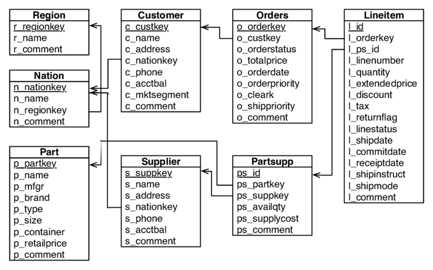

Honeydew models the schema as eight entities: customer, orders, lineitem, part, partsupp, supplier, nation, and region. Relations connect them in the same shape as the foreign keys in the warehouse.

Build the semantic model

Entities and relations

A Honeydew entity wraps a table in your warehouse. customer wraps the CUSTOMER table, orders wraps ORDERS, and so on. The entity declares its granularity key (the column or columns that make a row unique) and points at a source dataset that maps to the warehouse table.orders is the simplest shape, with a single-column key:

type: entity
name: orders
keys:
  - O_ORDERKEY
key_dataset: ORDERS

The matching type: dataset file binds ORDERS to the actual table: SNOWFLAKE_SAMPLE_DATA.TPCH_SF1.ORDERS on Snowflake, samples.tpch.orders on Databricks, or your own loaded copy.Some entities need more than one column as a key. lineitem is one row per line within an order, so its key is the order key plus the line number:

type: entity
name: lineitem
keys:
  - L_LINENUMBER
  - L_ORDERKEY
key_dataset: LINEITEM

Entities on their own don’t get you far. Insights come from connecting them, and that’s what relations are for: they tell Honeydew how entities JOIN, in which direction, and on which columns. lineitem is the central fact in this model. Every line item belongs to one order, so the relation from lineitem to orders is many-to-one:

type: entity
name: lineitem
keys:
  - L_LINENUMBER
  - L_ORDERKEY
key_dataset: LINEITEM
relations:
  - target_entity: orders
    rel_type: many-to-one
    connection:
      - src_field: l_orderkey
        target_field: o_orderkey

The rest follow the same many-to-one shape: lineitem to partsupp, orders to customer, customer and supplier to nation, nation to region, and partsupp to both part and supplier. Once the relations are declared, Honeydew handles the JOINs whenever a query mixes attributes from multiple entities.

Ask your coding agent: “Set up the TPC-H schema in my warehouse as Honeydew entities, with the relations between them.”

Metrics and attributes

A metric is an aggregation defined once at an entity’s granularity. Let’s start with revenue on lineitem. It’s the line-item price net of discount, summed across rows:

type: metric
entity: lineitem
name: revenue
description: revenue, as defined in TPC-H Q3, Q5 and others
datatype: number
sql: |-
  sum(lineitem.l_extendedprice * (1 - lineitem.l_discount))

Once it’s defined, you can group lineitem.revenue by orders.o_orderdate, customer.c_mktsegment, or nation.n_name, and Honeydew figures out the JOIN path from the relations you declared in the previous step.A calculated attribute is like a virtual column on an entity. TPC-H Q16 marks a supplier as having complaints when the supplier comment matches a pattern. Let’s codify that as a reusable attribute on supplier:

type: calculated_attribute
entity: supplier
name: has_complaints
description: For TPC-H Q16
datatype: bool
sql: |-
  supplier.s_comment like '%Customer%Complaints%'

Ask your coding agent: “On the supplier entity, add a boolean flag for whether a supplier has any customer complaints.”

Metrics also compose. TPC-H Q14 asks what share of revenue came from promoted parts. That’s a ratio metric on top of the revenue we already have:

type: metric
entity: lineitem
name: promo_revenue
description: Based on TPC-H Q14
datatype: number
sql: |-
  100.0 * lineitem.revenue FILTER (WHERE part.p_type LIKE 'PROMO%') / lineitem.revenue

FILTER (WHERE ...) scopes the inner revenue to line items where the part is a promotion. The JOIN through lineitem → partsupp → part to reach p_type is figured out by Honeydew. One expression, three tables.

Ask your coding agent: “On the lineitem entity, define total revenue using extended price net of discount. Then add a metric for the promotional share of revenue.”

See metrics and attributes for the reference. Recipes has more patterns: ratios, year-over-year growth, active-customer cohorts, and so on.

A domain

A domain is the part of the model that people and tools actually query. BI tools query domains. AI agents query domains. Domains can also apply mandatory filters and parameter overrides, so the full model stays broad while what a given consumer sees stays focused:

type: domain
name: orders_analytics
description: Orders, revenue and supplier analytics.

entities:
  - name: customer
  - name: orders
  - name: lineitem
  - name: part
  - name: partsupp
  - name: nation
  - name: region
  - name: supplier
    fields:
      - "*"               # all supplier fields, except...
      - "-s_comment"      # hide the raw comment column
      - has_complaints    # keep the derived flag

source_filters:
  - name: recent_orders
    sql: orders.o_orderdate >= '1992-01-01'
    description: Limit to orders inside the TPC-H data window.

source_filters apply only when the source entity is in the query; filters apply to every query on the domain. Domains can inherit from each other, so shared rules across finance, growth, supplier_ops, and other domains live in one place. See domains for both.

Ask your coding agent: “Create an orders_analytics domain that exposes the eight TPC-H entities, hides the raw supplier comment but keeps the has_complaints flag, and limits orders to 1992 onward.”

Run a query

Three ways to query the domain:

Honeydew Studio Playground: pick attributes and metrics interactively; the Playground shows the generated semantic query.
SQL: through the SQL interface, after connecting a BI tool or any JDBC client.
Coding agent: through the Honeydew MCP server.

Here’s the SQL form for “1997 revenue and promo share by region”:

SELECT
    "region.r_name" AS region,
    AGG("lineitem.revenue") AS revenue,
    AGG("lineitem.promo_revenue") AS promo_share_pct
FROM domains.orders_analytics
WHERE EXTRACT(YEAR FROM "orders.o_orderdate") = 1997
GROUP BY 1
ORDER BY 1

On the Snowflake TPC-H sample data, it returns:

region	revenue	promo_share_pct
AFRICA	6,492,190,414	16.59
AMERICA	6,757,276,923	16.51
ASIA	6,588,284,193	16.79
EUROPE	6,546,101,116	16.40
MIDDLE EAST	6,665,543,853	16.36

Add an AI layer

A context layer

The semantic layer captures what the data means. The context layer captures how your organization thinks about it: analytical methods, historical events, organizational knowledge, AI memory.A skill is a methodology the AI follows when a question matches its description:

---
type: instructions
subtype: skill
name: orders/revenue-drop-investigation
title: Revenue Drop Investigation
description: |-
  Step-by-step approach when revenue dips below the trailing
  three-month average. Use to localize the drop, compare promo
  vs non-promo revenue, check shipping delays, and cross-reference
  event context.
apply: on-demand
related_objects:
  - name: lineitem.revenue
    type: field
  - name: lineitem.promo_revenue
    type: field
---

# Revenue Drop Investigation

Use this skill when revenue dips below the trailing 3-month
average and the question is "why".

1. **Localize the drop.** Group `lineitem.revenue` by
   `customer.c_mktsegment`, `nation.n_name` and `region.r_name`.
2. **Compare promo vs non-promo.** Look at
   `lineitem.promo_revenue` in the same window.
3. **Check for shipping delays.** Compare `lineitem.l_shipdate`
   to `orders.o_orderdate`. A widening gap signals fulfillment
   issues, not demand.
4. **Cross-reference events.** Pull **Event** items whose
   `from_date`/`to_date` overlaps the drop window.
5. **Summarize.** State the most likely driver, the supporting
   evidence, and any alternatives that remain plausible.

Ask your coding agent: “Create a revenue-drop-investigation skill for the orders domain. It should walk the AI through localizing the dip by region and segment, comparing promotional vs non-promotional revenue, checking shipping delays, and cross-referencing historical events.”

An event is something that happened: a launch, a pricing change, an outage. When a question’s time range overlaps the event, the AI factors it into the analysis:

---
type: memory
subtype: event
name: 1997/q4-supplier-shortage
title: Q4 1997 supplier shortage
description: |-
  Regional supplier slowdown in EUROPE and ASIA causing shipping
  delays through Q4 1997. Depressed revenue and widened the gap
  between order date and ship date in the affected regions.
from_date: 1997-10-01
to_date: 1997-12-31
related_objects:
  - name: lineitem.revenue
    type: field
  - name: lineitem.promo_revenue
    type: field
---

A regional supplier slowdown across several nations in EUROPE and
ASIA caused shipping delays from October through December 1997.
Promotional campaigns underperformed because shipments slipped
past the promo end date. The gap between `orders.o_orderdate` and
`lineitem.l_shipdate` widened in the affected regions.

Ask your coding agent: “Record a Q4 1997 supplier-shortage event in EUROPE and ASIA. It caused shipping delays and depressed promotional revenue.”

Instructions, external knowledge from Notion or Confluence, and AI-generated decision traces round out the five context types. See context management.

An agent

An agent is where the domain and the context layer meet. It’s what users open in Honeydew Studio, Slack, Teams, or via MCP to ask a question:

---
type: agent
name: orders-analyst
display_name: Orders & Revenue Analyst
description: |-
  Investigates orders, revenue, promotions, and supplier patterns
  on the TPC-H demo model.
domain: orders_analytics
context:
  - orders/*
  - 1997/*
welcome_message: |
  Ask me about orders, revenue, promotions, suppliers or shipping
  patterns.
---

Use this agent to localize revenue patterns by market segment,
nation and region; evaluate promotion effects; and surface
shipping-delay patterns by comparing `lineitem.l_shipdate` to
`orders.o_orderdate`.

The TPC-H dataset spans 1992-01-01 through 1998-08-02 for orders;
ship dates run through 1998-12-01. Don't fabricate answers about
dates outside this window.

The same domain can back more than one agent. A supplier-ops-analyst could share the same orders_analytics domain with a different context set, for example.

Ask your coding agent: “Create an Orders & Revenue Analyst agent on the orders_analytics domain that loads context from the orders/ and 1997/ folders.”

Ask the AI

Open the orders-analyst agent and ask:

Anything notable about EUROPE and ASIA revenue patterns in late 1997?

Deep Analysis plans the investigation, runs a sequence of queries against orders_analytics, and uses the skill and event we just built. On the Snowflake TPC-H sample data, here’s what the agent comes back with:

EUROPE vs ASIA Revenue — Late 1997
Month ASIA EUROPE Leader
Jul $561M $552M ASIA
Aug $568M $560M ASIA
Sep $543M $533M ASIA
Oct $559M $559M tied
Nov $539M $540M EUROPE
Dec $560M $562M EUROPE
ASIA led consistently through Q3 with a ~$9–10M gap. October was a near-perfect tie. EUROPE pulled ahead in Q4, reversing the gap. The crossover from ASIA-dominant to EUROPE-dominant in late 1997 is the most notable finding.

Month	ASIA	EUROPE	Leader
Jul	$561M	$552M	ASIA
Aug	$568M	$560M	ASIA
Sep	$543M	$533M	ASIA
Oct	$559M	$559M	tied
Nov	$539M	$540M	EUROPE
Dec	$560M	$562M	EUROPE

Connect a BI tool

Connect orders_analytics to any supported BI tool. For programmatic access, use GraphQL or MCP.

What’s next

Modeling reference

Entities, relations, calculations, domains and advanced patterns.

Recipes

Cookbook for common metric shapes: ratios, year-over-year growth, active customers, nested aggregations.

AI Analyst

Deep Analysis, agents and the Context Layer in depth.

BI tool setup

Per-tool guides for Power BI, Tableau, Excel and more.

Quick Start

Semantic Ecosystem

Modeling Reference

Context Layer

Management

Integrations

Security

Release Notes

Where you’ll end up

What you’ll need

The data

Build the semantic model

Run a query

Add an AI layer

Ask the AI

Connect a BI tool

What’s next

Modeling reference

Recipes

AI Analyst

BI tool setup

​Where you’ll end up

​What you’ll need

​The data

​Build the semantic model

​Run a query

​Add an AI layer

​Ask the AI

​Connect a BI tool

​What’s next

Modeling reference

Recipes

AI Analyst

BI tool setup

Where you’ll end up

What you’ll need

The data

Build the semantic model

Run a query

Add an AI layer

Ask the AI

Connect a BI tool

What’s next